Stem-level forest inventory from a single aerial LiDAR flight. Individual location, DBH, height, and product class for every tree above threshold — verified against the source point cloud, repeatable across flights.
An Agcopter delivery includes a photographic 3D scene of the stand, an isolated stem cloud where every tree is individually located and measured, and a high-density bare-earth surface for forest-management use. Scroll to compare.
A photo-realistic 3D rendering of the stand — a Gaussian splat reconstruction from the same scan that produced the inventory. Pan, zoom, and walk through any part of the stand from a desktop browser, no LiDAR or GIS software required.
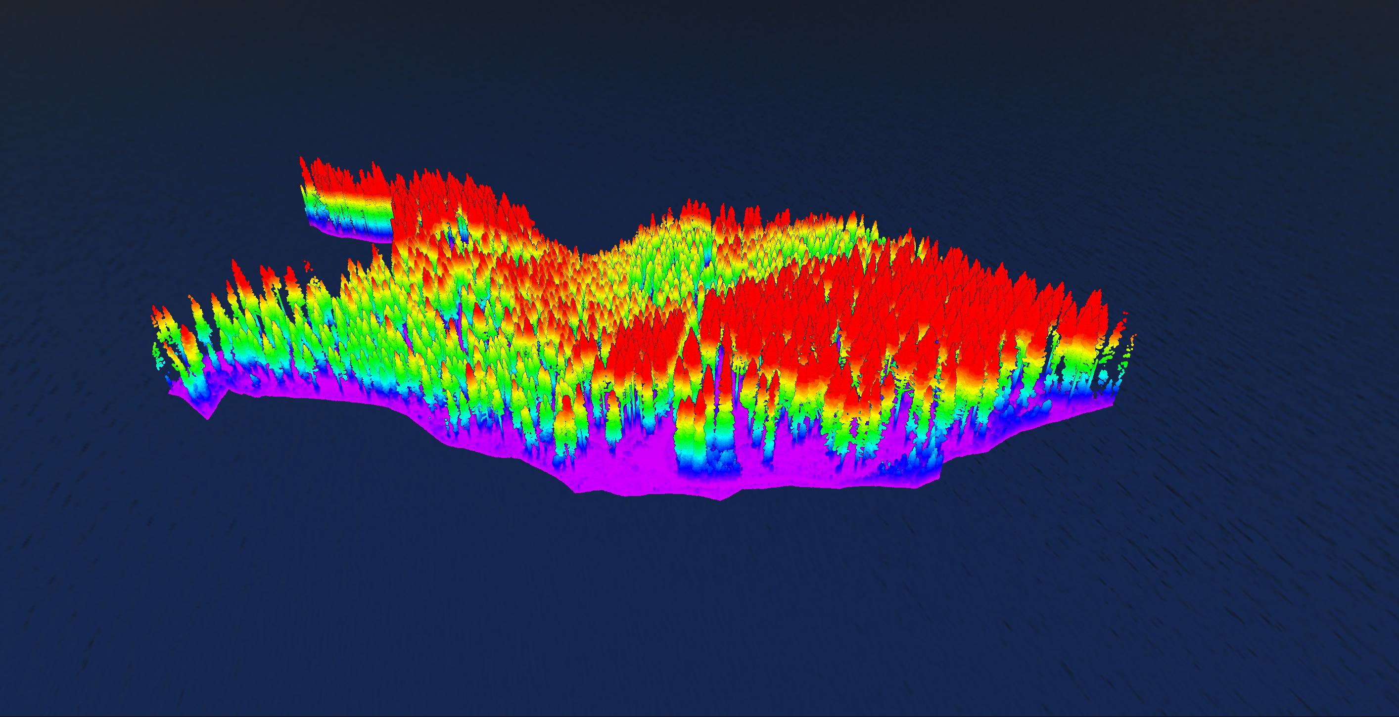
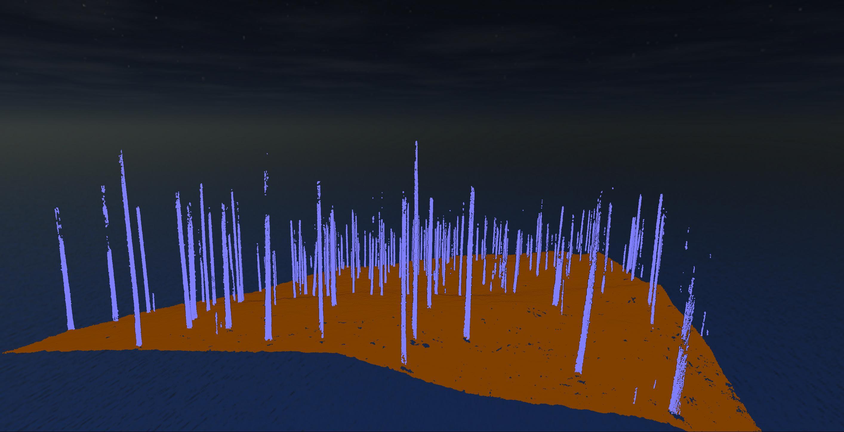
Each tree rendered as a colored cylinder — blue for shorter stems through yellow to red for the tallest. On the 70-acre pilot stand: 309 trees over 150 ft, including seven exceeding 180 ft. The canopy height model is delivered as crown-polygon shapefiles linked back to the stem inventory.
Each stem extracted from the LiDAR point cloud, separated from foliage and ground returns, then circle-fit at breast height (1.3 m) to measure DBH directly from the cloud. This is the geometry that produces the 1.5–2% DBH agreement against tape.
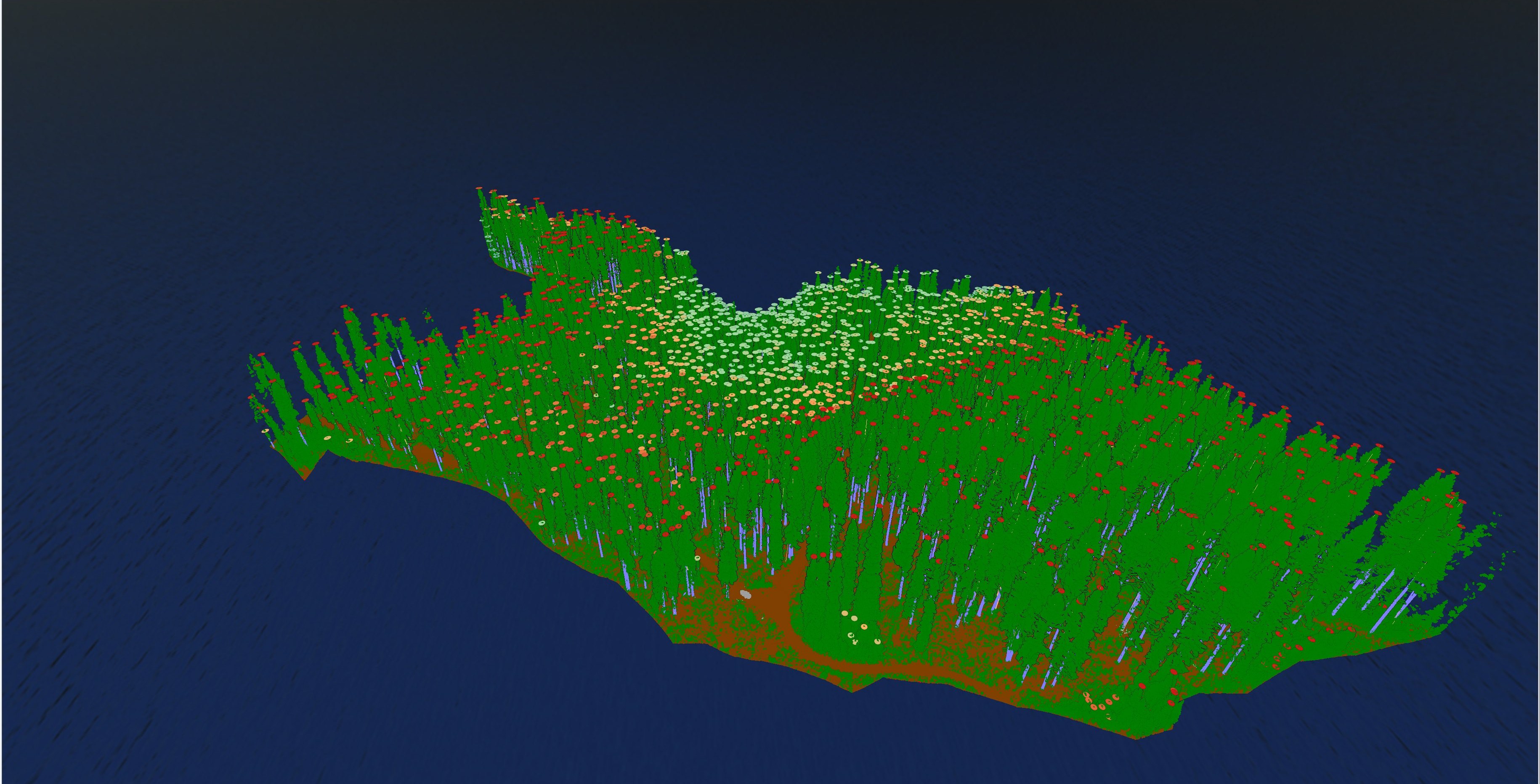
Crown polygons in green, isolated stems in purple. Each tree becomes a discrete record in the inventory with a persistent ID you can compare against future flights. Re-fly the same stand and growth, mortality, and disturbance are measurable per stem — not estimated from a sample plot.
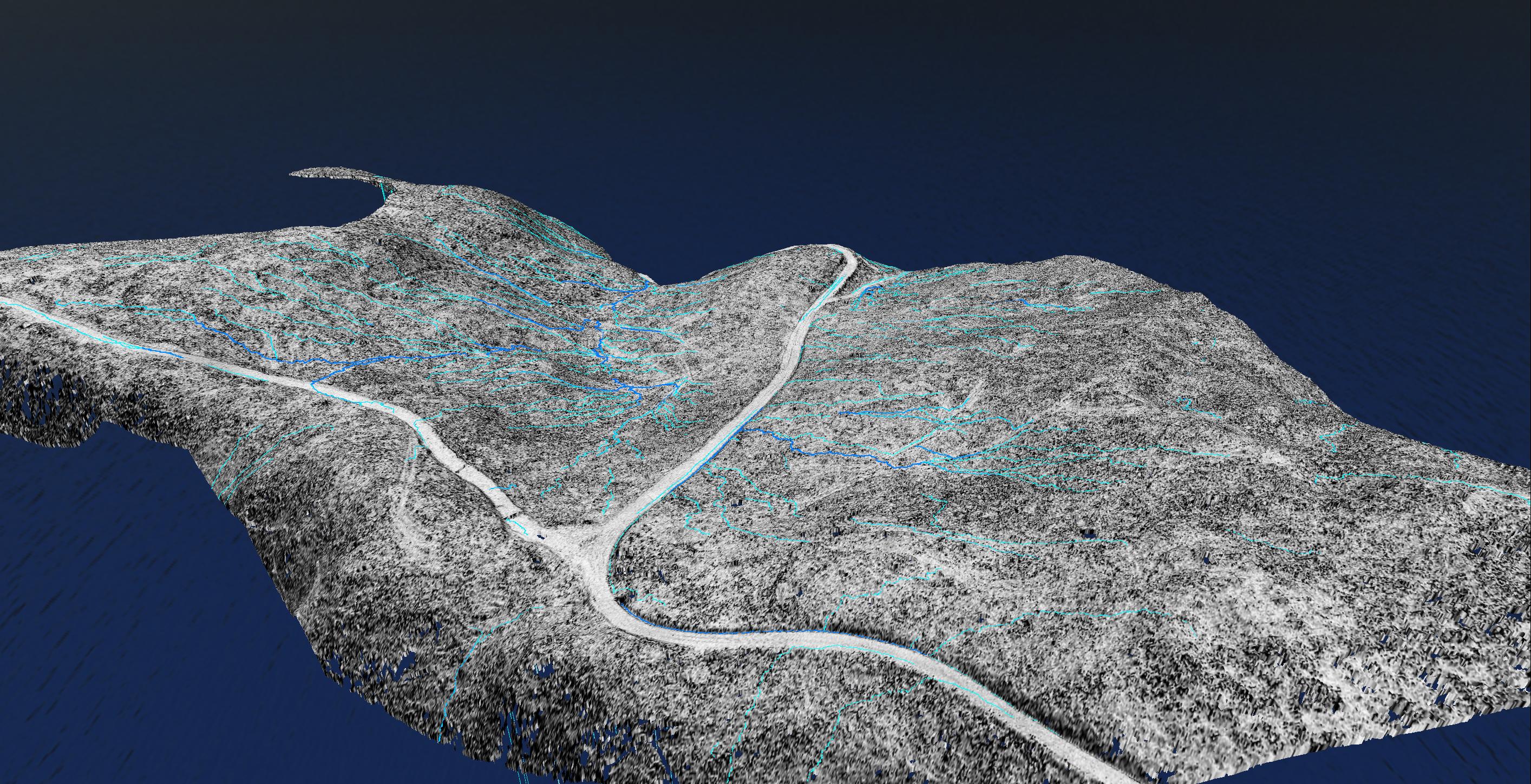
Bare-earth surface with synthetic drainage overlaid, delivered as supplemental input for forest-operations planning — road and skid-trail layout, riparian-buffer documentation, and stand-level slope review. Stamped topographic deliverables or engineered road / drainage designs stay with a licensed PE or PLS.
GIS-ready shapefiles, the source point cloud for independent verification, every chart in this report, and the same 3D scene your team will use for harvest planning.
CSV / shapefile / KML with DBH, height, crown area, lean, and product class. UTM Zone 10N or State Plane, stand-level location precision for in-field navigation.
Shapefile of per-tree crown polygons with height, area, and link back to the stem inventory. Reads directly as stocking pattern.
GeoTIFF raster plus synthetic drainage shapefile for forest-operations use — roads, landings, skid trails, riparian-buffer documentation, and stand-level slope review. Supplemental data; not a stamped topographic deliverable.
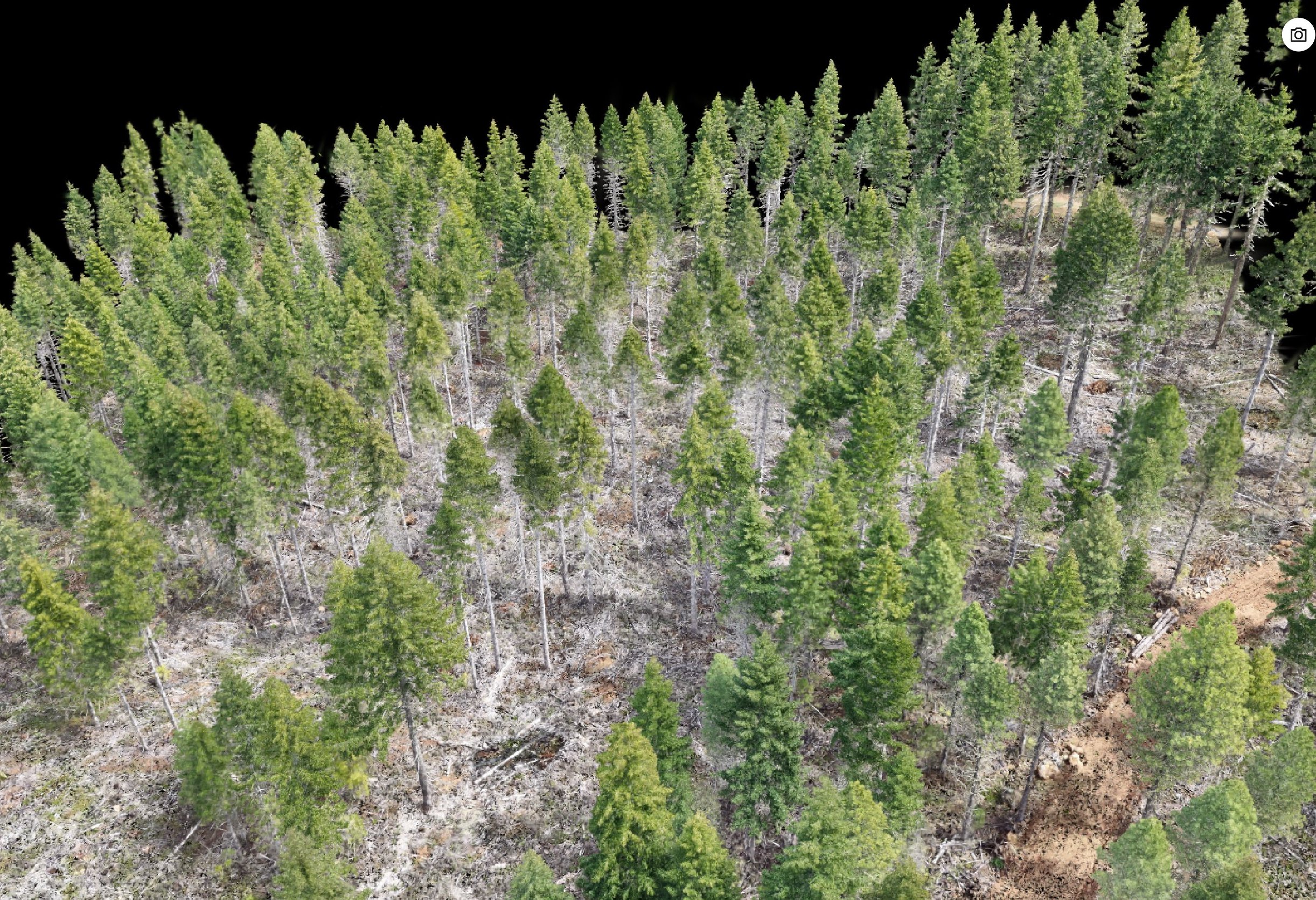
Photo-realistic Gaussian splat scene. Runs in a web browser with no LiDAR or GIS software. Useful for remote inspection and contractor briefings.
Embedded charts plus delivered spreadsheets. Feeds directly into cruise summaries, sale appraisals, and silviculture prescriptions.
LAZ format. Any tree in the inventory can be located and inspected directly — diameter, height, position, and surrounding stems all measurable in the cloud.
A photo-realistic reconstruction of the stand from the same scan that produced the inventory. Pan, zoom, and fly through every acre in a desktop browser — no LiDAR software, no installs. Useful for remote inspections, harvest planning conversations, and contractor briefings without a field visit.
Each row in the inventory is one physical tree. These attributes travel with it across the GIS layers, the spreadsheet, the KML, and any future re-flight of the same stand.
Same tree, identifiable on any future flight — growth, mortality, recruitment measurable per stem.
Diameter at breast height with a circle-fit chi-squared metric flagging stems where the geometry is ambiguous.
Tree height plus crown polygon area and within-crown height percentiles P10–P90.
Vertical profile of the stem — supports merch volume, pole-length screening, and bucking plans.
From the 3D trunk axis vector. Supports felling-direction planning and wind-damage cluster identification.
Pulpwood through peeler. Anomaly flags: snag, broken-top, lean, multi-stem, pole candidate.
How many other trees share the same canopy polygon. 0 = alone in its crown; ≥1 = co-dominant cluster.
UTM Zone 10N or State Plane. Stand-level location precision — sufficient to navigate to every stem on the cruise tablet.
Every flagged anomaly and resolution is documented in the QC log delivered with the report. No stems dropped without explanation.
A wall-to-wall stem-level inventory of a thinned 70-acre stand anchored by medium and small sawtimber, with 296 peeler-class stems carrying about 40% of the basal area.
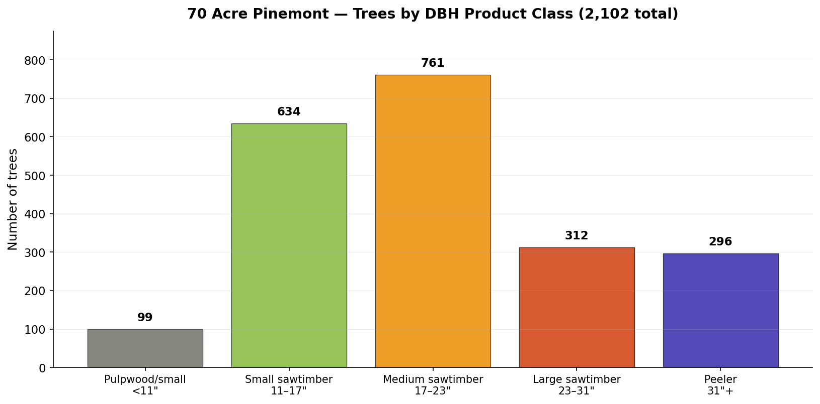
Medium sawtimber (17–23") is the largest cohort at 761 stems — 36% of the inventory. The 296 peeler-class stems at 31"+ are 14% of stems but a disproportionate share of basal area.
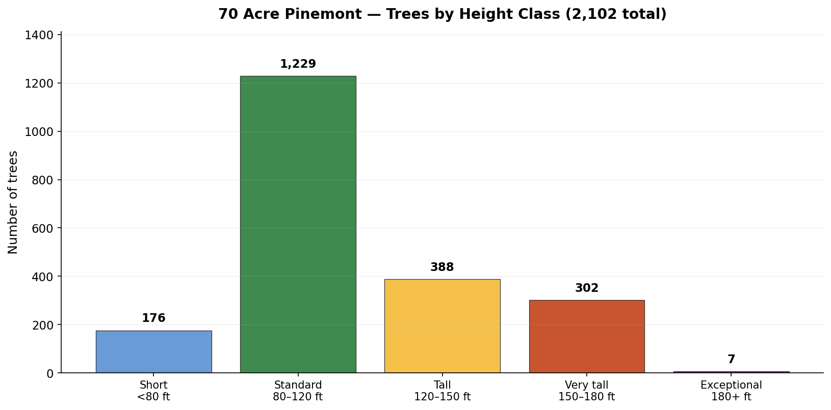
Standard-height trees (80–120 ft) account for 1,229 stems — the dominant cohort left after thinning. 309 trees are over 150 ft tall, including seven exceeding 180 ft.
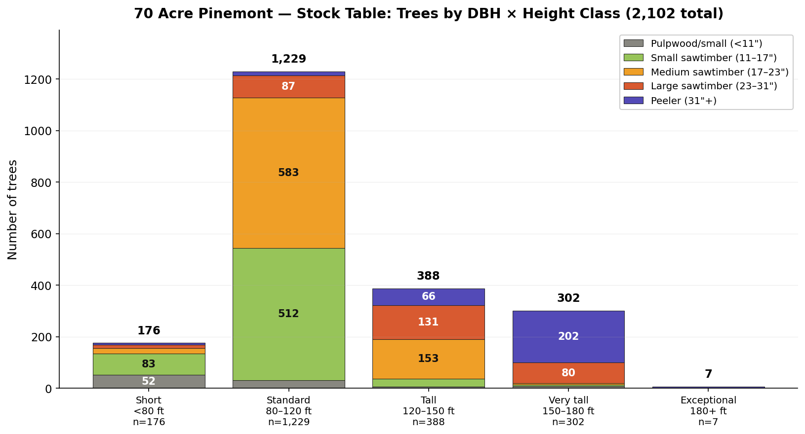
The two-dimensional matrix single-axis charts can't show. The largest single cell is medium sawtimber × standard height at 583 trees.
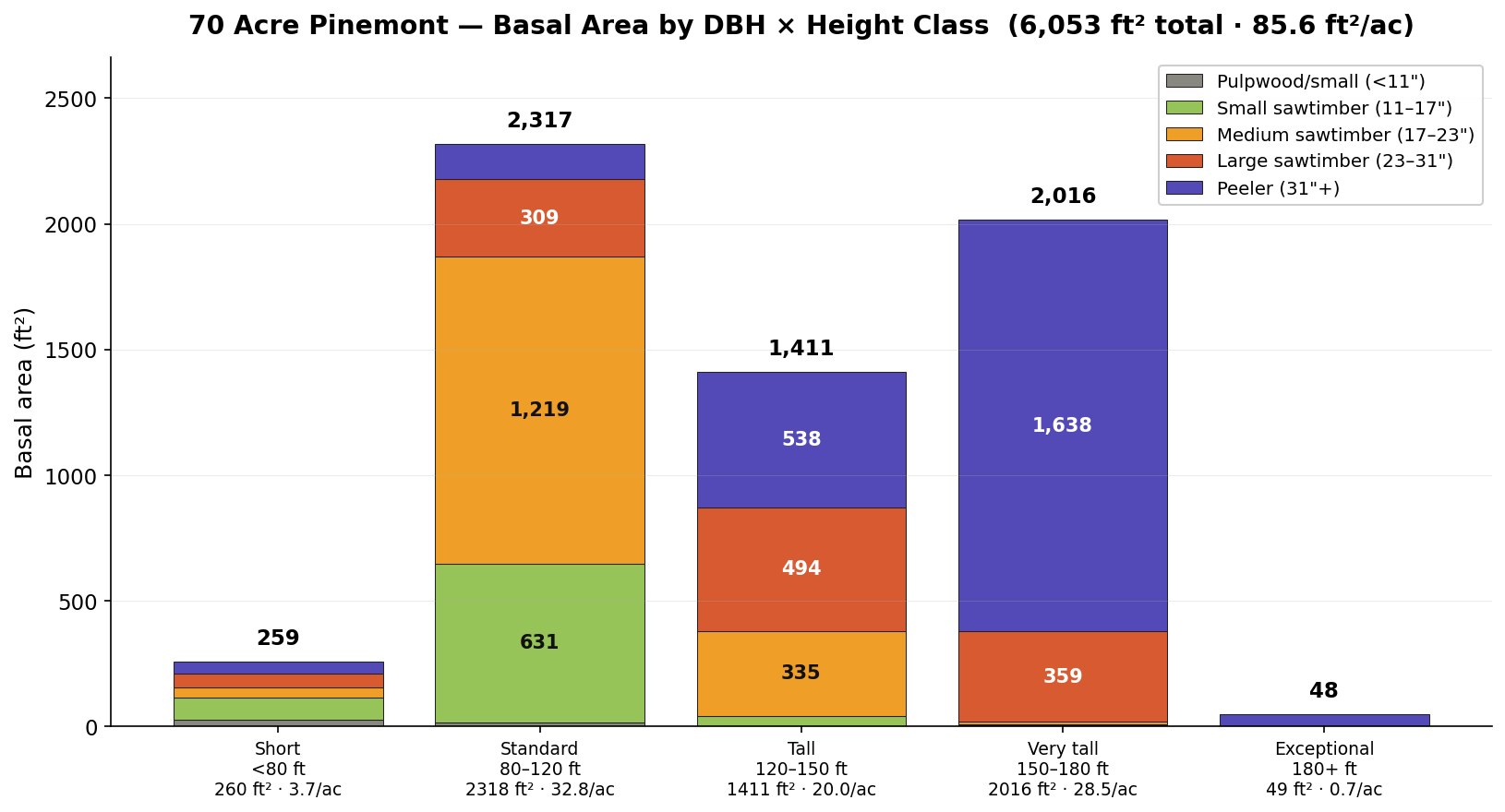
Same matrix, weighted by basal area. The single largest cell is peeler × very-tall — 1,638 ft² of BA in 202 stems, more than any other size combination.
A traditional plot cruise reports stand averages and expansion factors from a 10–20% sample. Agcopter measures the population directly, then delivers GIS-ready shapefiles, the source point cloud, and a verifiable record of every stem.
Cruisers record structural features as subjective field notes when they record them at all. Agcopter computes them from the per-tree geometry — every flagged stem has a precise location and is included in the delivered GIS layer for field follow-up.
Maximum measured lean: 39.1°. 111 stems lean more than 5°. Computed from the 3D trunk axis vector — supports felling-direction planning and wind-damage cluster identification.
Flagged as more than 1.5σ shorter than DBH-predicted height. Catches standing dead snags, wind-snap survivors, broken tops — many worth retaining as wildlife snags, some worth recording for salvage.
Sharing a crown polygon with at least one neighbor (18% of inventory), including 56 in clusters of three or four. Each carries a shared_crown_count attribute so users can filter or weight accordingly.
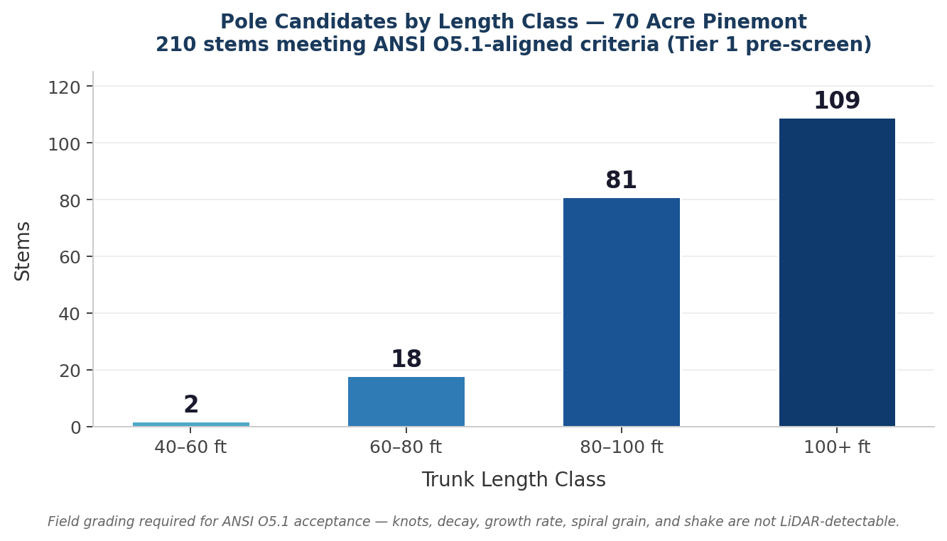
Meet all five LiDAR-measurable ANSI O5.1 criteria simultaneously. Field grading still required for knots, decay, growth rate, spiral grain, and shake — these aren't assessable from aerial LiDAR.
Each candidate passes simultaneously: DBH 10–25", trunk length > 40 ft, lean < 1.0° from vertical, lower-bole sweep within 1" per 10 ft of length (multi-slice circle-fit centers), and circle-fit r_redchi < 1×10⁻⁵ indicating sound geometry at breast height.
The dominant tier is 100+ ft — transmission-class poles commanding the highest per-unit premiums. The 80–100 ft class covers the most commonly traded distribution lengths. The lean and bole-sweep filters do significant work: a loose pre-filter without sweep returns 1,339 candidates; the ANSI-calibrated criteria reduce that by 6×.
All 210 candidates delivered as a separate KML layer, color-coded by length class.
The inventory finds the trees. The field-route deliverable tells your forester how to walk them. Every flagged stem — pole candidates, leaners, snags, multi-stems — exported as a KML/KMZ with a travelling-salesman-optimized inspection route. Loadable into OnX Hunt, Avenza, or any GPS field app. Hours of bushwhacking saved on every visit.
Save your TSP route screenshot to img/tsp-route.jpg and this placeholder will swap to your actual deliverable preview.
On the 70-acre pilot, 210 stems passed ANSI O5.1 pre-screen criteria. Inspecting them all on foot in random order means hours of backtracking. The Agcopter deliverable solves the routing for you: the shortest walking path that hits every stem.
Two independent ground-truth checks anchor the inventory. The source point cloud is delivered with the report — any tree can be located and inspected directly by the forester.
22 trees on the 70-acre stand were measured with a diameter tape and compared against their LiDAR-fitted DBH from two separate flights. Agreement is within the variability of tape measurements themselves.
15 trees out of 2,117 candidates required correction during QC; 2,102 retained. All 15 errors at the top of the DBH distribution where stems physically touch — the regime where any inventory method has the most trouble.
Trees between 11" and 30" DBH with clean fits showed no detected errors. For comparison, conventional cruising might report 5–15% sampling error at the stand level depending on plot density.
Verifiability. The point cloud is delivered with every report. Any tree in the inventory can be located and inspected by the forester directly — diameter, height, position, and surrounding stems are all measurable in the cloud. On the pilot stand, flight-to-flight measurements of the same stems agreed within 1.5–2% across separate days, demonstrating the consistency required for any meaningful monitoring use of the system over time.
The per-stem inventory, canopy structure, and structural attributes on this page are forest mensuration deliverables for forest-management decision-making — stocking, harvest planning, riparian-buffer documentation, regulatory reporting, and timber valuation. The bare-earth terrain and drainage products are high-density supplemental data for forest-operations planning.
They are not, and are not delivered as, certified topographic mapping, engineered grading or drainage design, stamped survey deliverables, or legal boundary work. Where a stamped or certified deliverable is required — boundary survey, engineered road or drainage design, regulatory submission — we partner with a licensed PE or PLS in responsible charge.
Quotes are scoped per stand based on acreage, terrain, and deliverables. Currently flying Pacific Northwest forests.